For a number of years now I have, from time-to-time, made the odd stab at trying to find the flowline of a river from the mapped surface area of the watercourse using OpenStreetMap data.
 |
| Windermere in the English Lake District, one of my test cases. |
I not infrequently find, being neither trained as a geospatial specialist nor a mathematician, that, although I have a fairly clear idea of what I want to do with some particular manipulation of geodata, I am stymied. More often than not this is simply because I don't know the most widely used term for a particular technique. It was therefore really useful to learn from
imagico that the generic term for what I was trying to do is
skeletonisation. (I do hope my relative ignorance is not on
this scale.)
Armed with this simple additional piece of knowledge immediately opened out the scope of resources available to me from wikipedia articles, blog posts, to software implementions. Unfortunately when I first tried to get the relevant extensions (
SFCGAL) installed in PostGIS I was not able to get them to work, so I shelved looking at the problem for a while.
Very recently I re-installed Postgres and Postgis from scratch with the latest versions and the
SFCGAL extensions installed fine. So it was time to re-start my experiments.
Once I was aware of skeletonisation as a generic technique I also recognised that it may be applicable to a number of outstanding issues relating to post-processing OpenStreetMap data. Off the top of my head & in no particular order these include:
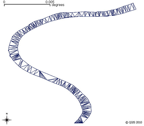 |
My earliest experiment using Ordnance Survey Open Data for the River Trent
Voronoi triangles based on modes of polygon, clipped back to polygon |
- Waterway flowlines. Replacing rivers mapped as areas by the central flowline where such a flowline has not already been mapped. Such data can then be used for navigation on river systems or for determining river basins (and ultimately watersheds/hydrographic basins). (It is this data which much of the rest of the post is concerned with).
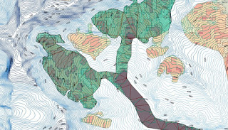 |
Earlier experiments with OpenStreetMap glacier data for the Annapurna region
Height (contours) & slope(shading) data via Viewfinderpanorams.com
Voronoi triangulation clipped to glacier used to try & find flowlines for the main Annapurna Glacier.
Some ideas originated from conversations with Gravitystorm.
Map data (c) OpenStreetMap contributors 2014. |
- Glaciers. Similarly for rivers although height also needs to be factored in. The idea is not just to identify flows on a glacier, but also simulate likely regions of higher speed flow with a view to creating an apparently more realistic cartographic depiction of the glacier. (Only apparent because in reality one needs lots of good aerial photography to correctly map ice-falls, major bergschrunds, crevasses, crevasse fields etc.).
- Creating Address Interpolation lines. A small subset of residential highways have quite complex structures and therefore it is non-trivial to add parallel lines for address interpolation. Buffering the multilinestring of the highway centre lines & then resolving that to a single line would help. (More on this soon).
- Dual Carriageways. Pretty much the same issue as above except there is the additional problem of pairing up the two carriageways. Resolving them to a single way would make high-level routing and small scale cartography better (i.e., it's a cartographic generalisation technique).
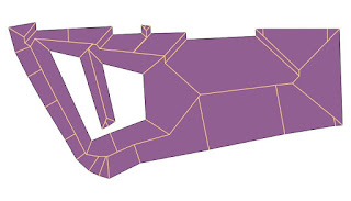 |
The straight skeleton of Old Market Square Nottingham which allows routing across and close to most of the square
The skeleton does not take account of some barriers on the square,
but the hole at the left (a fountain shows the principle).
Data source: (c) OpenStreetMap contributors 2015. |
- Routing across areas for pedestrians. Pedestrian squares, parks car parks etc. Skeletonisation of such areas may offer a quick & dirty approach to this problem.
What follows are some experiments I've done with water areas in Great Britain. I have mainly used the
ST_StraightSkeleton function, with rather more limited time spent looking at
ST_ApproximateMedialAxis. The two images below show my initial attempt to find hydrographic basins: this works merely by chaining together continuous waterway linestrings. These results are not bad, but several major rivers are divided into multiple watersheds. The map of Ireland shows the problem better because the Shannon system appears as a number of discrete watersheds, largely because the Shannon flows through a number of sizeable lakes. Other major rivers illustrating the issue in the UK are the Dee, Trent and Thames.
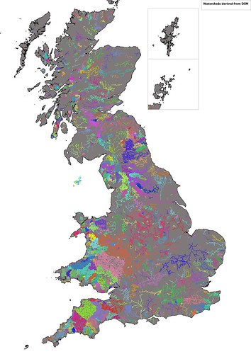 |
| Identification of watersheds in Great Britain by contiguous sections of waterway in OpenStreetMap |
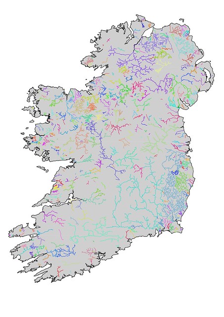 |
Watersheds in Ireland derived from linear watercourses on OpenStreetMap.
Waterways are generally less well-mapped in Ireland, but also several major waterways pass through large lakes (e.g., the Bann (Lough Neagh), Shannon (Lough Ree, Lough Derg), and the Erne (Upper & Lower Lough Erne)) and no centre line is available. |
So the naive approach raised two problems:
- Lakes, rivers mapped as areas etc also needed to be included in creating the elements of the watershed
- Actual watersheds can be created by creating Concave shells around their constituent line geometries.
Unfortunately I get a PostGIS non-noded intersection error when trying this, so wont discuss it further (although if someone can walk me through how to avoid such problems I'm all ears). As later versions of PostGIS seem more robust I return to this later.
Of course the simple way to address the first one is just to include areas of water as additional objects in the chain of connected objects. However I would also like to replace rivers as areas, and smaller lakes with linestrings as this type of generalisation can greatly assist cartography at smaller scales. The lack of a source of generalised objects derived from OSM has been a criticism of its utility for broader cartographic use, so this is another aspect of this investigation.
So now with skeletonisation routines working in PostGIS time to look at some of the basics.
I've taken Windermere, the largest lake in England, as an example to work through some of the issues. Windermere is a long thin lake which should have a fairly obvious median line. However, it does have some islands which complicate the matter.
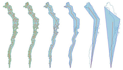 |
Six versions of Windermere showing area, media axis (red), straight skeleton (thinner lines)
for different degrees of simplification (parameters of 0,5,25,125..).
Original shape is shown as a blue outline.`
All created as a single query using st_translate. |
Both the straight skeleton & the medial axis are complicated multi-linestrings if I use raw OSM data for Windermere. Progressive simplification of the shape reduces this complexity with reasonable desirable medial axis appearing when simplified with the parameter of around 100 (assumed to be meters in Pseudo-Mercator). Unfortunately there are two problems: the derived axis passes through large islands; and inflow streams are not connected.
I therefore took a different approach. I disassembled Windermere using ST_Dump and cut the line forming the outer ring at each point a stream or river way touched the lake. I then simplified each individual bit of shoreline between two streams & then re-assembled the lake.
When this is done all inflows & outflows are connected to the straight skeleton of the simplified lake area. This can be input directly into my routines for collecting all ways making up a watershed.
Additionally the straight skeleton can be pruned. The simplest one is to just remove all individual linestrings which dangle (i.e., are not connected to a waterway). Presumably one can iterate this until one has the minimum set necessary to a connected set of flows, but I haven't tried this.
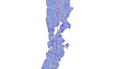 |
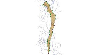
Straight Skeletons for Windermere calculated for different simplification parameters.
The grey lines represent a parameter where details of islands are kept but the number of edges in the skeleton is greatly reduced. |
 |
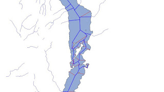
| Windermere showing inflow & outflow waterways | | |
 |
| Detail of the centre of Windermere showing a reduced straight skeleton linked to inflowing streams (blue). The equivalent without reassembly and preserving stream topology is in red |
For a single lake it is possible to determine the appropriate degree of simplification to apply, but the complete set of lakes & ponds in Great Britain is a completely different matter.
Over simplification will result in too big a discrepancy between the original shape and adjacent geometries. Even for Windermere trying to include islands in a reassembly fails with too great a degree of simplification because geometries now cross each other.
My approach has been to simplify geometries with parameters from 50 to 250 metres in ST_Simplify. I then compare a number of factors with the original:
- Do I get a valid geometry
- Number of interior rings
- A measure of surface area
With these I then choose one of the simplified geometries for further processing. In general large lakes and riverbank polygons will tolerate more simplification. The overall result is less complicated straight skeletons for further processing. (As an aside I think
Peter Mooney of Maynooth did some work on comparing lake geometries using OSM data around 2010 or 2011).
For my immediate practical purposes of finding watersheds I did not perform further pruning of skeletons, but such a process is needed for other applications such as cartographic generalisation.
Even with my first approach which I thought was fairly robust I'm losing a fair number of waterways with simplification. I haven't looked into this further because it will delay finishing this particular post: and it's been on the stocks long enough.
For further posts on the problems of skeletonisation read
Stephen Mathers blog which I found very useful.
StyXman is
developing a JOSM plugin which uses some of these techniques to create centrelines too. A big thank you to him, and, of course, to Christoph Hormann (
imagico).